
studio.heelab
[DL for CV] Regularization & Optimization 본문
Lecture: https://www.youtube.com/watch?v=dyNGd06MWn4&list=PLoROMvodv4rOmsNzYBMe0gJY2XS8AQg16&index=3
1. Regularization
Adding an extra term to the loss function to prevent the model from overfitting to the training data. The goal is to improve performance on unseen test data (generalization) even if it slightly reduces training performance.
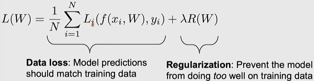
hyperparameter (Lambda): A value that controls the strength of regularization; 0 means no regularization, and higher values apply stronger regularization.

- L2 Regularization (Weight Decay): Adds the sum of squared weights to the loss, encouraging the model to spread out the weight values evenly.
- L1 Regularization: Adds the sum of absolute weight values, inducing sparsity in the weight matrix (driving many values to zero).
2. Optimization Basic
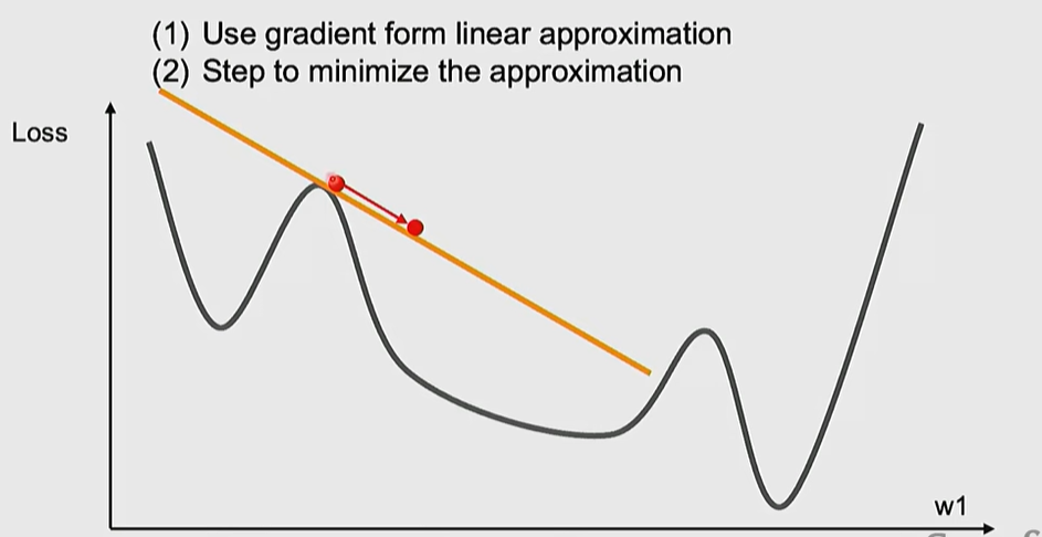
Loss Landscape Analogy: Optimization is the process of finding the lowest point (minimum loss) in a complex terrain. It is similar to a blindfolded person hiking down a mountain by only feeling the gradient (slope) beneath their feet.
Calculating Gradients
Numerical Gradient
-approximate, slow, easy to write
Calculated manually by adding a tiny value $h$ using the limit formula. It is easy to implement but very slow and only an approximation.
Analytic Gradient
-exact, fast, error-prone
Derived exactly using calculus (e.g., the Chain Rule). it is fast and precise.
Gradient Descent
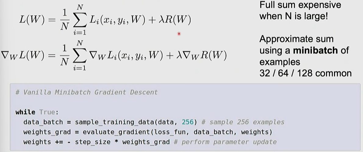
#Vanilla Gradient Descent

while True:
	weights_grad = evaluate_gradient(loss_fun, data, weights)
    weights += -step_size * weights_grad #perform parameter update
3. Optimizers
SGD (Stochastic Gradient Descent)
Calculates gradients and updates parameters using only a randomly sampled mini-batch instead of the entire dataset
Problem 1:
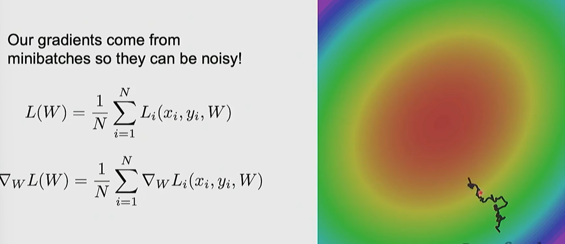
When the loss function has uneven curvature across different dimensions (high condition number), SGD suffers from excessive jitter along steep directions and painfully slow progress along shallow ones.

Problem 2:
Oscillations in narrow/deep valleys and getting stuck at local minima or saddle points.

Problem 3:
Sample only a subset of the data
Advanced Algorithms:
Momentum
: Maintains a velocity from previous updates to use inertia, helping escape local minima/saddle points and smoothing out noise.
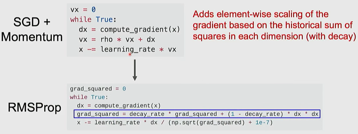
RMSProp
: Scales the learning rate for each parameter based on the magnitude of the gradient—moving slower in steep directions and faster in flat directions.
Adam
: Combines the advantages of Momentum and RMSProp; it is the most widely used default choice in modern deep learning.
AdamW
: An improved version of Adam that handles weight decay separately for better regularization.

4. Learning Rate

Learning Rate Scheduling: The technique of gradually decreasing the learning rate as training progresses.
Learning rate decays over time
Reduces the learning rate by a factor (e.g., 1/10) at specific intervals.
usually using in ResNet

Learning Rate Cosine Decay
Smoothly decreases the learning rate following a cosine curve.

Linear Warm-up
Starts with a low learning rate, gradually increases it, and then decreases it.

Linear Scaling Rule: A practical rule stating that if you increase the batch size by n you should also increase the learning rate by n
1st order Optimization
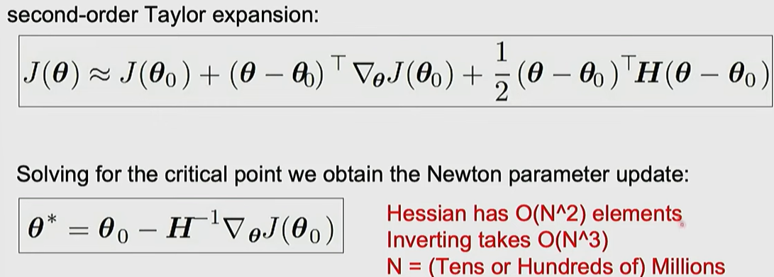
2nd order Optimization

* Practical Advice: When tackling a new problem, start with AdamW as the default and apply either a constant learning rate or a cosine scheduler
'MMAILab' 카테고리의 다른 글
| [DL for CV] Training CNNs and CNN Architectures (0) | 2026.03.05 |
|---|---|
| [DL for CV] Image Classification with CNNs (0) | 2026.03.05 |
| [DL for CV] Neural Networks & Backpropagation (0) | 2026.03.04 |
| [DL for CV] Image Classification with Linear Classifiers (0) | 2026.03.04 |
| [DL for CV] Introduction (1) | 2026.03.04 |


