
studio.heelab
[DL for CV] Neural Networks & Backpropagation 본문
Lecture: https://www.youtube.com/watch?v=25zD5qJHYsk&list=PLoROMvodv4rOmsNzYBMe0gJY2XS8AQg16&index=4
1. Basic Structure of Neural Networks
Neural networks: the original linear classifier -> 2layers
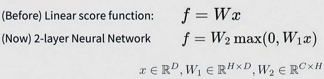

Multi-layer Structure: Beyond a single linear layer (W x X), neural networks are constructed by stacking multiple layers, such as W_2 x max(0, W_1 x X).
Hidden Layers: Intermediate neurons learn specific features (templates) of the data. For example, individual neurons can capture partial features of an object, such as an animal's eyes or legs.
Nonlinearity: If a non-linear function is not inserted between linear transformations, stacking multiple layers ultimately reduces to a single linear function. Thus, non-linear transformation is crucial.
2. Activation Functions
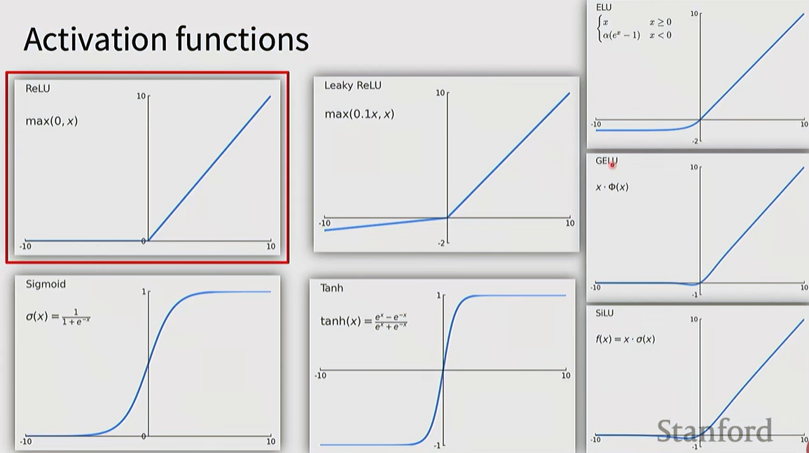
ReLU (Rectified Linear Unit): The most widely used default choice.
Various Variants:
Leaky ReLU / ELU: Used to solve the "Dead Neuron" problem of ReLU.
GELU / SiLU (Swish): Frequently used in Transformers and modern CNN architectures.
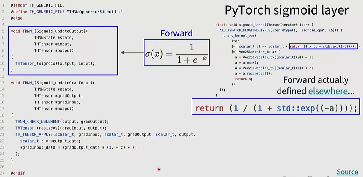
Sigmoid / Tanh: These squash values into a specific range, but can cause the Vanishing Gradient problem when used in intermediate layers; therefore, they are primarily used near the output layer.
Selection Criteria
Mostly empirical; it is recommended to first use functions that have been proven in existing architectures.
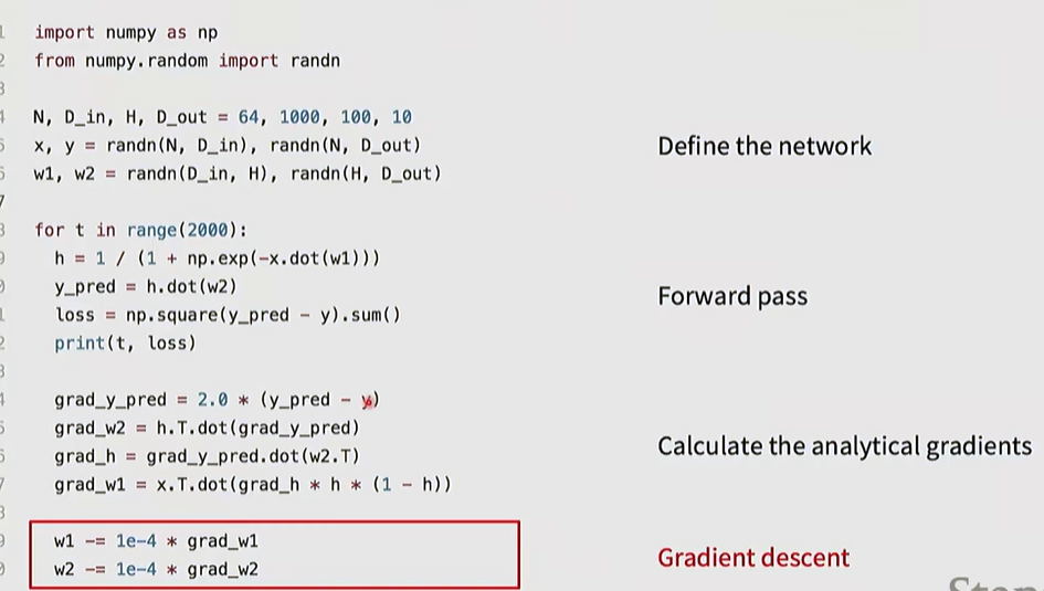
3. Practical Neural Network Design and Training
Full implementation of training a 2-layer Neural Network needs ~20 lines
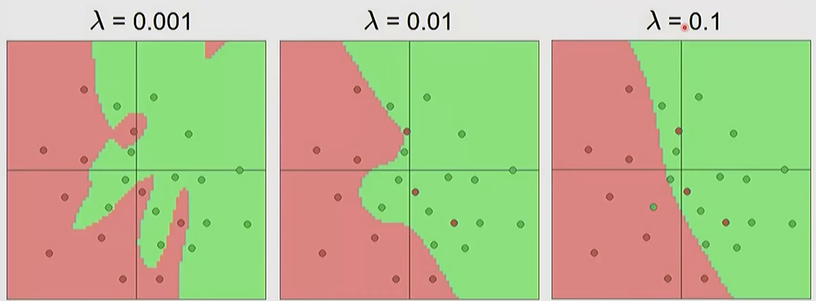
Setting the number of layers and their sizes

Model Capacity: A higher number of neurons allows the model to learn more complex functions, but increases the risk of overfitting.
Hyperparameter Tuning: A common practice is to use a sufficiently large network and prevent overfitting by adjusting the regularization (\lambda) strength, rather than shrinking the network size itself.
Biological Inspiration: Neural networks are loosely inspired by the structure of actual brain neurons (cell body, dendrites, axons), but actual biological mechanisms are far more complex
Plugging: how to compute gradients

4. Computational Graphs and Backpropagation

Computational Graphs: Complex functions are visualized as step-by-step operational nodes to facilitate derivative calculations.
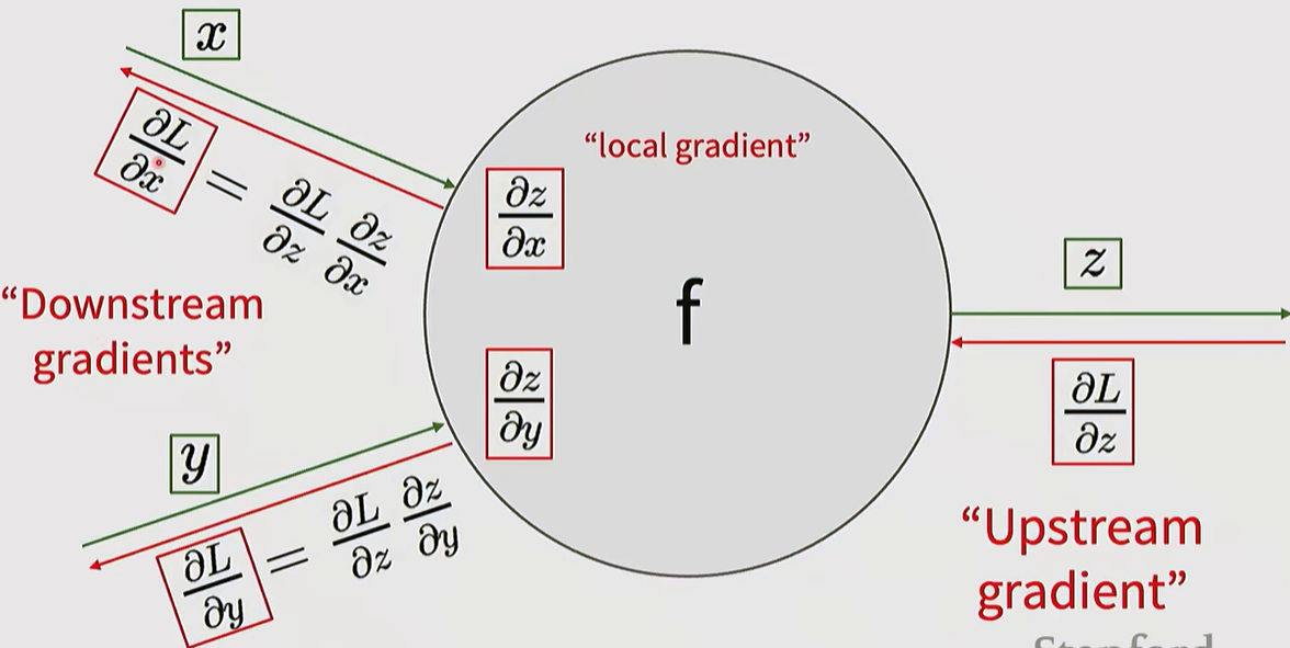
Backpropagation Principle: Gradients are propagated from the output (Loss) toward the input by applying the Chain Rule.
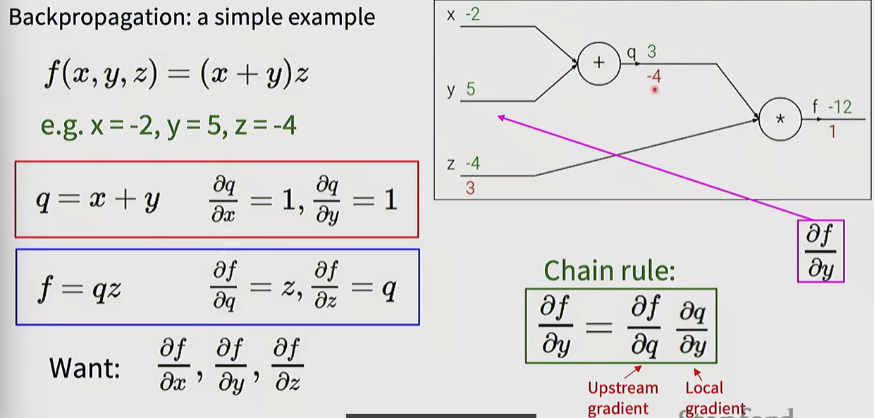
- Upstream Gradient: The gradient passed back from the succeeding node.
- Local Gradient: The derivative of the output with respect to the input at the current node.
- Downstream Gradient: The value passed to the preceding node, calculated by multiplying the Upstream and Local gradients.
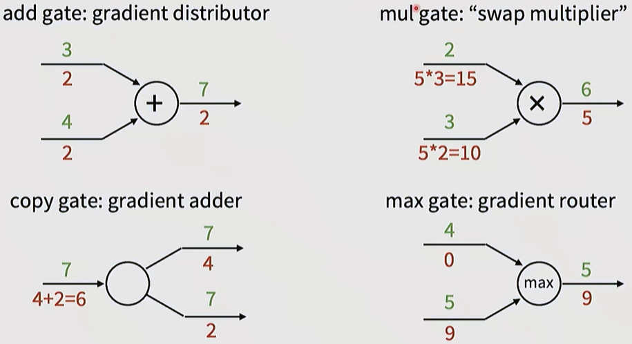
Characteristics of Major Operational Nodes:
- Add gate: Acts as a distributor, passing the gradient through unchanged.
- Multiply gate: Acts as a swap multiplier, multiplying the gradient by the swapped input values.
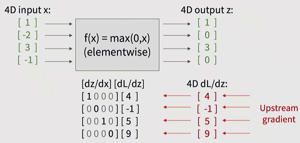
- Max gate: Acts as a router, passing the gradient only to the path with the higher value.
Patterns in gradient flow
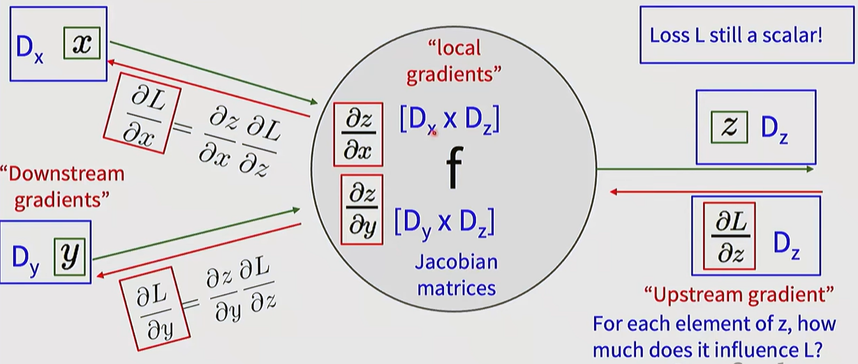
5. Backpropagation in Vector and Matrix Operations
Vectorization: Actual implementations process data in units of vectors and matrices rather than scalars. In this case, the local gradient takes the form of a Jacobian Matrix.
Efficiency: Instead of storing massive Jacobian matrices (which could exceed 256GB) in memory, calculations are performed efficiently using matrix calculus formulas (e.g., the derivative of X x W involves multiplications with their respective transposes).
Back with Vectors
'MMAILab' 카테고리의 다른 글
| [DL for CV] Training CNNs and CNN Architectures (0) | 2026.03.05 |
|---|---|
| [DL for CV] Image Classification with CNNs (0) | 2026.03.05 |
| [DL for CV] Regularization & Optimization (0) | 2026.03.04 |
| [DL for CV] Image Classification with Linear Classifiers (0) | 2026.03.04 |
| [DL for CV] Introduction (1) | 2026.03.04 |


